Feature Timing, Predicting When Features Will Work

I hear from @arbitrage that a number of the users on top of the leaderboard have high feature exposure to just one feature or may in fact simply be setting their entire submission to be one feature like feature_intelligence1.

It’s tempting to say this is crazy and will result in big burns but is it possible that feature timing can be achieved and done well and reliably and that people staking with lots of exposure to one feature are not crazy?

One potential way to argue that feature timing doesn’t work is if features move in a random way. As in a feature is just as likely to be >0 correlation with the target as it is to be <0 correlation regardless of the recent history of the feature… i.e. the feature performance is memoryless: it’s like betting on black or red in roulette… 7 reds in a row doesn’t make black more likely (or red more likely for that matter).

So if you look at the feature scores per era for every era, do their scores have the statistical property that they look like roulette or do they appear to have non-random “runs” or “regimes” which can’t be explained by chance?

If they don’t behave randomly, are they model-able and can we say things like “now is a good time to have a little be extra feature exposure to feature_intelligence1”.

One test I like for randomness is the Wald–Wolfowitz runs test - Wikipedia but I lost my Python code of it.

Another easier one is auto-correlation. If you score every feature vs the target by itself and then compute the autocorrelation, you find that some features have large positive or negative autocorrelation. For example, “feature_wisdom27” has 0.24 autocorrelation. Positive autocorrelation means if it’s had good performance lately it will tend to continue to have good performance (long runs). Negative autocorrelation means it’s mean reverting.

If feature_wisdom27 has had >0 performance with the target four eras in a row, how much would you stake that it will have a fifth >0 performance next? How could you build a model to give you good probability estimates of what will happen next so you can use those to inform your stakes?

TARGET_NAME = f"target"
PREDICTION_NAME = f"feature_intelligence1"

# Submissions are scored by spearman correlation
def correlation(predictions, targets):
    ranked_preds = predictions.rank(pct=True, method="first")
    return np.corrcoef(ranked_preds, targets)[0, 1]

# convenience method for scoring
def score(df):
    return correlation(df[PREDICTION_NAME], df[TARGET_NAME])

data["eraNum"] = data["era"].apply(lambda x: int(x[3:]))
feature_names = [
        f for f in data.columns if f.startswith("feature")
    ]

def ar1(x):
    return np.corrcoef(x[:-1], x[1:])[0,1]

for f in feature_names:
    feature_per_era_corrs = data.groupby('eraNum').apply(lambda d: correlation((d["target"]), (d[f])))
    print(f)
    print(ar1((feature_per_era_corrs>np.mean(feature_per_era_corrs))*1))

feature_wisdom27_per_era_corrs = data.groupby('eraNum').apply(lambda d: correlation((d["target"]), (d["feature_wisdom27"])))
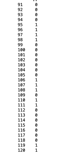
(feature_wisdom27_per_era_corrs>np.mean(feature_wisdom27_per_era_corrs))*1

feature_wisdown27 runs:
13 Likes

Beware of all this factor timing is called a sin at AQR and they ain’t great at it when they sin… maybe works better on our abstract features but maybe not.

5 Likes

Just wanted to chime in here. Some background: I am the submitter of the i3 model. I wanted to do a proper post about this after collecting some more information, I still will do this but I wanted to point out some of the potential pitfalls of this post now to avoid any unnecessary burns. First, by my calculations feature_wisdom27 has an autocorrelation much lower than the 0.24 stated in this post, in fact when I calculated this it seems statistically insignificant. Second, looking at just runs of positive or negative correlations can be misleading, for example if a feature has a 0.9 probability of staying the same sign with a correlation of +/-0.005 and a 0.1 probability of flipping sign and getting a correlation of +/-0.05, then this isn’t something you want to stake on (kind of similar to the buy the dip mentality, it works until it doesn’t). Also a small self plug but I’m going to be speaking to @arbitrage about this and other things (including some potential pitfalls of feature neutralisation) on OHwA this Thursday, if anyone wants to ask me any questions about it hop on and I’ll do the best I can to answer :slight_smile:

6 Likes

looking forward to hearing what you have to say to arbitrage and your post on this.

the way I calculated autocorrelation here was first creating a series of whether wisdom27 was above it’s mean performance or not and then computing the autocorrelation of that.

if I compute ar1(feature_wisdom27_per_era_corrs) the autocorrelation is lower like you say at 0.0837.

importantly: I’d definitely not recommend these types of methods to beginners – better to first become an expert at creating models that work well in all regimes before going down this dangerous rabbit hole.

3 Likes

I’m fairly new to NumerAI and I’m still testing the model I’ve developed (round 254 is my second week submitting results from the completed model) but I think it has promise. My method involves sifting out noisy features while leaving the most regularly significant features. I won’t include my code because it’s pretty inefficient and novice, but here’s the process in principle:

Step 1: Sample the same number of rows per unique era (anywhere from 1 to 26 rows per era). Using only the training dataset that’s anywhere from 120 to 3,120 samples. The reason for this is to avoid intra-era correlation

Step 2: Divide the number of total sampled rows by 10 to determine the maximum number of features to regress on the target; the number 10 comes from the rule of thumb that you need at least 10 samples per variable in a regression. Then you randomly select that number of features for a regression. (e.g. say you sample 5 rows per era, that’s 600 samples. You’d randomly select 60 out of the 310 features to regress on the target)

Step 3: Run an OLS regression on the target using the sample rows and sample features.

Step 4: Record the pvalues for each feature in the regression.

Step 5: Repeat steps 1 - 4 ten-thousand times.

What you end up with is a list of features and pvalues about 1.6 million rows long. I have two methods of sifting this data:

Method 1
Filter out every instance where a feature received a pvalue < 0.01. Every feature will achieve this pvalue a few times after 10,000 random regressions but there is a probability distribution with the number of occurrences you can expect any feature to obtain this pvalue in 10,000 regressions.

P(feature_x being selected in a regression) = (12 + 310) / (2 * 310) = 161 / 310 = 0.5194
P(feature_x pvalue < 0.01 | due to error) ≈ 0.01 (conservative estimate)

Expected number of times feature_x achieves pvalue of < 0.01 due to error in 10,000 regressions = 0.01 * 0.5194 * 10,000 ≈ 52 times.

Here is the probability distribution function:
f(x) = (10,000 choose x) * (1.61/310)^x * (308.39/310)^(10,000-x)

Then filter out any features that did not achieve a pvalue of 0.01 at least 64 times out of the 10,000 regressions. In theory this should filter out 95% of the features leaving you with ~16 significant features.

Method 2
Take the average pvalue of every feature and select the 16 features with the lowest average pvalues.


You can obviously change parameters to select more or less features within these methods. What I am currently doing is selecting ~100 features per method and then keeping the features which appear in both lists (which is usually around 60 features).

Then you simply remove the features that didn’t make the cut from the training dataset and train your preferred MLA with that dataset. The idea is that you’re training your model using features which are, on average, correlated most to the target. If you adjust the parameters to select less features you are exposed a lot to the most significant features. If you adjust the parameters to include more features, you are less exposed to any one feature but are introducing noise to the model.

Finding the middle ground is a matter of speculation, though a self-correcting algorithm could optimize the number of feature to select.

5 Likes

I would be interested on your view on out of sample correlation and (smart) sharpe.
If your sharpe is good, then this would mean there is no info in the pruned features that make the model less risky in the validation data, which would surprise me.

Also: If you want to evaluate your model I have read several times that a era-fold cross validation on training+validation and checking especially for eras with negative correlation is a good measure.

I think this paper might be helpful to detect the regime.
Geometric Dataset Distances via Optimal Transport

The paper suggests that they can measure the distances between datasets.
In numerai tournament, this might be useful to detect the datasets which are near the live data.
As a result, the effective features might be detected from these datasets near the live era.

The implementations are here:

5 Likes

Am I wrong or that (interesting!) paper deals datasets with labels? In that case, we cannot use otdd to live data…

Every time I’ve tried something like measuring distances between eras with different methods (with the old dataset anyway), the result is always the same. The oldest eras start out wherever they are and then the data gradually changes era-by-era, i.e. eras are similar to their nearby neighbors in time and that’s pretty much it. And no indication you can predict where the targets are going to go based on that (even when the targets abruptly shift, there is no special detectable disturbance in the data that era), and eras far apart in time are far apart in distance (so you can’t go “oh this era looks like some era 5 years ago, the results will be similar”). Maybe others have better luck with such schemes, or the new dataset doesn’t act this way? (Doubt it, but haven’t checked.)

Still, it is interesting information. You might think at first that with all the regularization they do, that the eras would all be kind of the same (in a way) and detectable differences between them might be significant prediction-wise. Alas, no. It seems to be the case that the eras do have a “signature” to them, but it only seems to be a signature in time and not especially useful for prediction. But again, others may be more clever or have made better discoveries…

5 Likes