Performing Exploratory Data Analysis on Numerai Tournament Data with R

theomniacs · November 18, 2020, 5:39pm

Numerai is a crowdsourced hedgefund that hosts tournaments, which attract thousands of data scientists around the world to compete for Numeraire cryptocurrency. The company provides clean, regularized, and obfuscated data, where anyone with expertise in machine learning can freely participate. Other than that, they also include various guides and coding samples to help novice data scientists get started. One way to get the data is simply visit https://numer.ai/.

In this article, we will perform exploratory data analysis on the numerai_training_data.csv using R to find out more about each feature and the target. In a recent development, starting for round 238 opening on November 14th, 2020 the official target will migrate from “Kazutsugi” to the newer “Nomi”. In preparation for the migration, we’ll perform our analysis on the new Nomi target.

The Data

The training_data is 1.3 GB and contains information on 501808 rows across 314 columns. The first three columns are as follow:

‘id’ – an unique identifier of each row
‘era’ – a time period corresponding to a trading day
‘data_type’ – indication of whether the row is part of train/test/validation/live

These three columns are then followed by 310 features columns and the last column for the target. Our very first observation of the data is that all the feature columns and the target column take on only 5 numeric values: 0, 0.25, 0.5, 0.75, and 1. Below shows a sample of the first few columns and rows.

See Code

id	era	data_type	feature_intelligence1	feature_intelligence2	feature_intelligence3	feature_intelligence4
n000315175b67977	era1	train	0.00	0.5	0.25	0.00
n0014af834a96cdd	era1	train	0.00	0.0	0.00	0.25
n001c93979ac41d4	era1	train	0.25	0.5	0.25	0.25

The features are categorized into 6 categories: intelligence, charisma, strength, dexterity, constitution, and wisdom. Note that these categories are not of the same size. There are 12 “Intelligence”, 86 “Charisma”, 38 “Strength”, 14 “Dexterity”, 114 “Constitution”, and 46 “Wisdom” variables. Let’s now take a look the summary statistics of these features.

Table: Data summary


Name	features
Number of rows	501808
Number of columns	310
_______________________
Column type frequency:
numeric	5
________________________
Group variables	None

Variable type: numeric

skim_variable	complete_rate	mean	sd	p25	p50	p75	p100	hist
feature_intelligence1	1	0.5	0.35	0.25	0.5	0.75	1	▇▇▇▇▇
feature_intelligence2	1	0.5	0.35	0.25	0.5	0.75	1	▇▇▇▇▇
feature_intelligence3	1	0.5	0.35	0.25	0.5	0.75	1	▇▇▇▇▇
feature_intelligence4	1	0.5	0.35	0.25	0.5	0.75	1	▇▇▇▇▇
feature_intelligence5	1	0.5	0.35	0.25	0.5	0.75	1	▇▇▇▇▇

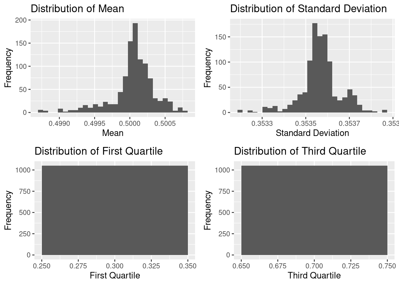
We see in the data that all the columns are in the correct format, the data is clean and ready for analysis. There are no missing value and from first glance, many of the features share similar distributions. Histograms of the actual values point to an almost universal uniform distribution across each variable, the distributions of the summary statistics appear to be either normally distributed or heavily skewed.

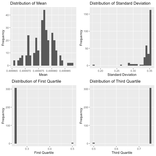
It seems that the mean and median of every feature are very close to 0.5. Most of the features have standard deviation around 0.35, while there are a few with exceptionally low standard deviations of less than 0.2. Almost all of the features have their first quartile and third quartile exactly on 0.25 and 0.75 respectfully. A few of them have first quartile and third quartile curiously at 0.50.

How do these distributions look for each feature category? Let’s find out:

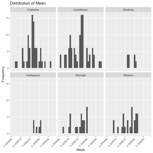
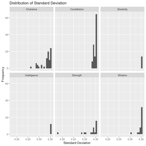
We note that outliers seem to appear in the “Strength” and “Charisma” categories. Let’s look more closely to find out which ones.

Table: Data summary


Name	features
Number of rows	501808
Number of columns	310
_______________________
Column type frequency:
numeric	4
________________________
Group variables	None

Variable type: numeric

skim_variable	complete_rate	mean	sd	p25	p50	p75	p100	hist	category
feature_strength20	1	0.5	0.18	0.5	0.5	0.5	1	▁▁▇▁▁	Strength
feature_strength38	1	0.5	0.18	0.5	0.5	0.5	1	▁▁▇▁▁	Strength
feature_charisma25	1	0.5	0.27	0.5	0.5	0.5	1	▂▂▇▂▂	Charisma
feature_charisma47	1	0.5	0.27	0.5	0.5	0.5	1	▂▂▇▂▂	Charisma

We can see that feature_strength20 and feature_strength38 are the ones that have the lowest standard deviation (almost half the norm). It is also very interesting that all of the outliers come from two categories: “Charisma” and “Strength”.

Though we have many features, they are all symmetrical and they look like one of the following types.

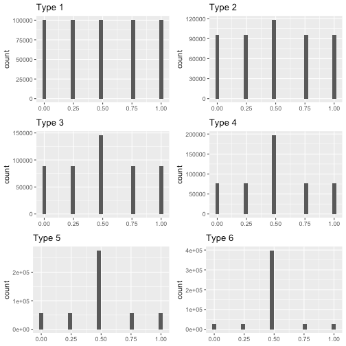
Type 1 is uniform distribution and Type 2 to Type 6 are simply various degrees of spread (measured by standard deviation) centered at 0.5. Note that Type 5 and Type 6 are the outliers we mentioned earlier.

We see that the two smallest categories: “Intelligence” and “Dexterity” all have Type 1. “Strength” and “Charisma” have a mix of almost all the types.

Here is a frequency table showing exactly how many of each category is of each Type.

category	Type 1	Type 2	Type 3	Type 4	Type 5	Type 6	Total
Charisma	22	24	24	14	2	0	86
Constitution	62	22	30	0	0	0	114
Dexterity	14	0	0	0	0	0	14
Intelligence	12	0	0	0	0	0	12
Strength	14	6	10	6	0	2	38
Wisdom	30	12	2	2	0	0	46
Total	154	64	66	22	2	2	310

How about the target value? Let’s take a look at it’s summary statistics:

skim(training_data['target'])

Table: Data summary


Name	training_data[“target”]
Number of rows	501808
Number of columns	1
_______________________
Column type frequency:
numeric	1
________________________
Group variables	None

Variable type: numeric

skim_variable	n_missing	complete_rate	mean	sd	p0	p25	p50	p75	p100	hist
target	0	1	0.5	0.22	0	0.5	0.5	0.5	1	▁▃▇▃▁

The target does not belong to any of the aforementioned Types. The distribution looks like a normal distribution.

Pearson Correlation Coefficient

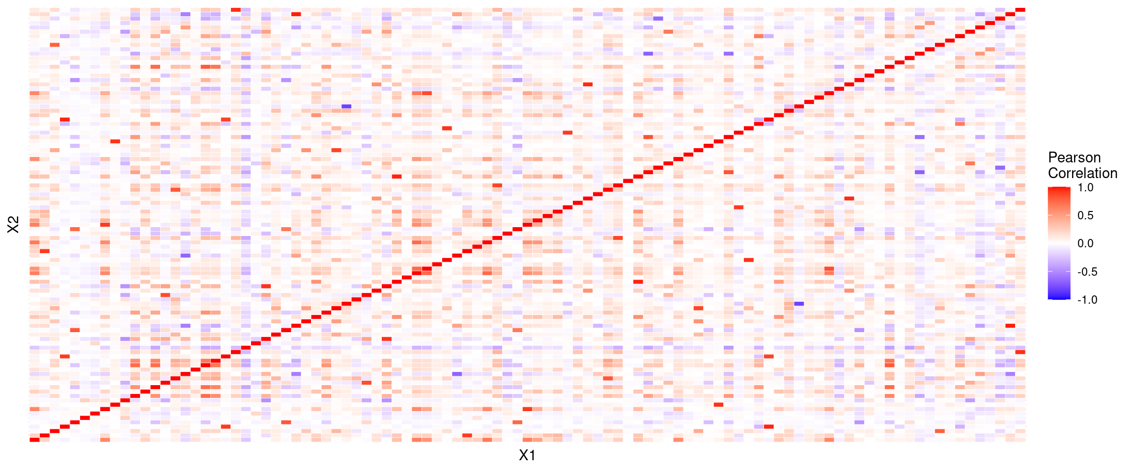
We now take a look at the correlations between the features.

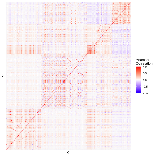
Though it is not easy to get much out of the heatmap, we can sort of see that features within each category, they are mostly correlated (some are negative correlated) with each other.

X1	X2	value	absvalue
feature_wisdom12	feature_wisdom2	0.97	0.97
feature_wisdom2	feature_wisdom12	0.97	0.97
feature_wisdom46	feature_wisdom7	0.96	0.96
feature_wisdom7	feature_wisdom46	0.96	0.96
feature_charisma69	feature_charisma9	0.95	0.95

The table confirms that features within the same category are highly correlated with each other (mostly positive correlated). We also see that some features in “Intelligence” are highly correlated with some features in “Dexterity”. For example:

feature_dexterity1 and feature_intelligence10 have correlation 0.82
feature_dexterity3 and feature_intelligence2 have correlation 0.82
feature_dexterity8 and feature_intelligence3 have correlation 0.81

On the other hand, we noticed that there are many features that have 0 correlation with each other, and it is surprising that some of them belong to the same category. For example, feature_constitution3 has zero correlation with 14 other features in the same category.

We can also explore correlations between linear combinations of features within the same category. Here, we can use equal weighted linear combination (i.e. mean) of the features within each group. Below shows the correlations heatmap:

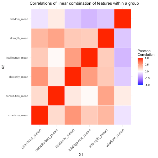
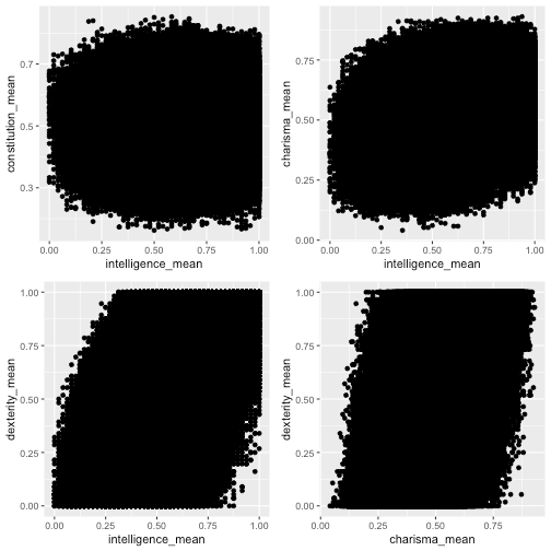
We can see that the linear combination of “Intelligence” has no correlation with “Constitution” (0.01). Another interesting observation is that “Dexterity” are moderately correlated with both “Intelligence” and “Charisma” (0.5 and 0.55 respectively) but “Intelligence” and “Charisma” are not very correlated (0.27). We can see the relationships with the scatter plots as well.

When we look at the correlations between the features and the target, we see that all of them are not correlated with the target. The highest correlation of 0.01/-0.01 with the target. This simply implies that the features do not have a linear relationship with the target. What it does not imply is that the features have no relationship with the target.

X1	X2	value	absvalue
target	target	1.00	1.00
feature_intelligence2	target	-0.01	0.01
feature_intelligence3	target	-0.01	0.01
feature_charisma1	target	0.01	0.01
feature_charisma2	target	0.01	0.01

As expected, when we look at correlations between linear combinations of features and the target, we see that none of them are correlated with the target.


intelligence_mean	0.00
charisma_mean	0.01
strength_mean	0.01
dexterity_mean	-0.01
constitution_mean	0.00
wisdom_mean	0.01

Scatter Plots

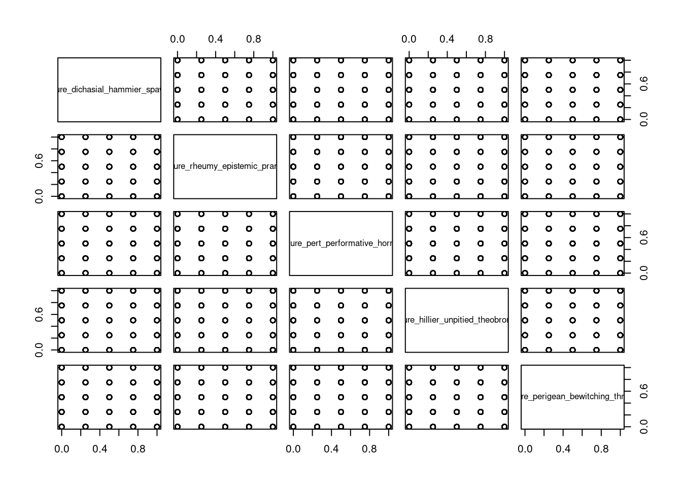
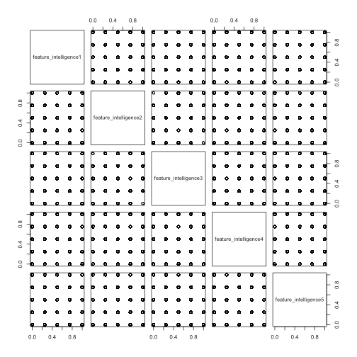
Looking at many of the scatter plots, almost all of the scatter plots look like the following, even the ones with high correlation. Unfortunately, we are not able to say much about the features from the scatter plots other than they have taken almost all possible combinations of values in the data.

pairs(intelligence[1:5])

Mosaic Plots

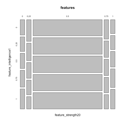
Let’s explore some mosaic plots. For instance, going back to the outlier we discussed, this mosaic plot shows that feature_strength20 are heavily centered at 0.5 while feature_intelligence1 is evenly distributed at each value.

mosaicplot(~feature_strength20+feature_intelligence1,data=features)

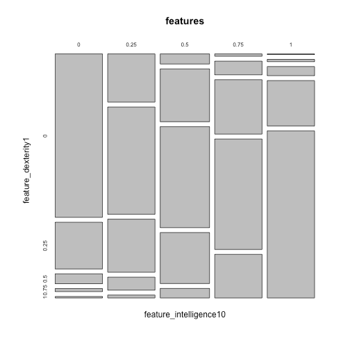
Here is another interesting mosaic plot where it clearly shows that there is a strong correlation between feature_intelligence10 and feature_dexterity1, which we have seen while we looked at correlations.

mosaicplot(~feature_intelligence10+feature_dexterity1,data=features)

Principal Components Analysis

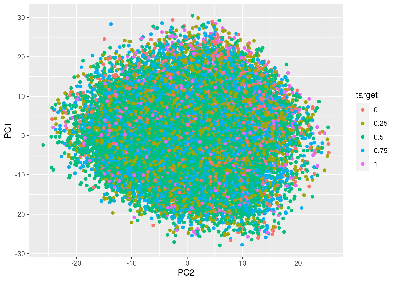
Since we have many features, principal component analysis could be useful. We see that the first 50 principal components will be able to explain 82% of variance, which is not bad considering we started from 310 features.

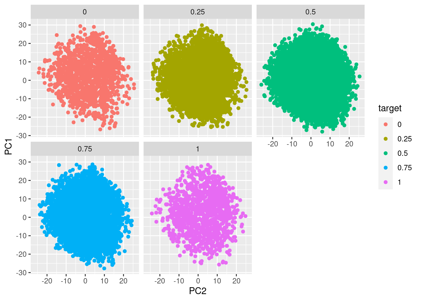
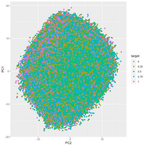
Here are two plots of PC1 vs PC2, where no clear clusters can be seen. Notice that similar situation occurs across the rest of the components as well. We can only conclude that the target value exists all across different inputs, which is unfortunate as it implies predicting the target could be a difficult task.

Conclusion

From the analysis, we found that many of the features are very similar to each other and even though there are 6 categories of features, there are no clear distinction between them. Here are some interesting things we found:

50% of the features and the target are uniformly distributed.
“Charisma” and “Strength” features are the categories that vary the most in their distribution.
Many features within the same category are highly correlated with each other. However, there are also features within the same category that have zero correlation.
“Dexterity” is moderately correlated with both “Intelligence” and “Charisma”, which suggests that dimension reduction is likely to play a significant role in the modeling process.
Due to the discrete structure of the features and target, the scatter plots we produced were not very helpful.

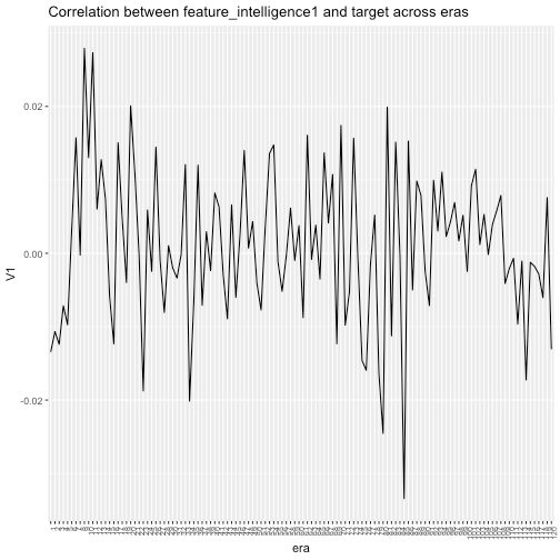
We also found that none of the features are correlated with the target, which was indeed very curious; however, when performing the same analysis across different eras we found trends that inspired our next post analyzing time dependencies in the dataset. We leave you with the following example of the correlation between feature_intelligence1 and the target across eras where we clearly see the relationship is a function of time.

References

Numerai Sample Scripts – [https://github.com/numerai/example-scripts]
New Target Nomi Release – [New Target Nomi Release]
Numerai [https://numer.ai/]
Numerai – Wikipedia [https://en.wikipedia.org/wiki/Numerai]

liz · July 11, 2021, 2:10am

this was dope, surprised it had no discussion on it. thanks for the exploration!

autratec · July 11, 2021, 1:04pm

Amazing analysis. Good job.

theomniacs · December 2, 2021, 9:03pm

With the release of the Super Massive Dataset, we’ve finally got around to updating our previous exploratory analysis in hopes it gives some of our Numerai newcomers a quick run down of what they can expert when modeling this data.

The Data

The training_data is 10.7 GB and contains information on 2,412,105 rows across 1074 columns. The first two columns are as follow:

‘era’ - a time period corresponding to a trading day
‘data_type’ - indication of whether the row is part of train/test/validation/live

These three columns are then followed by 1050 features columns, the target column as well as 20 more target columns, and an identifier column. Our very first observation of the data is that all the feature columns and the target column take on only 5 numeric values: 0, 0.25, 0.5, 0.75, and 1. Below shows a sample of the first few columns and rows.

## # A tibble: 3 × 7
##   era   data_type feature_dichasial_ha… feature_rheumy_epis… feature_pert_perfo…
##   <chr> <chr>                     <dbl>                <dbl>               <dbl>
## 1 0001  train                       1                   0.5                 1   
## 2 0001  train                       0.5                 1                   0.25
## 3 0001  train                       0.5                 0.25                0.75
## # … with 2 more variables: feature_hillier_unpitied_theobromine <dbl>,
## #   feature_perigean_bewitching_thruster <dbl>

Previously, the features were categorized into 6 categories: intelligence, charisma, strength, dexterity, constitution, and wisdom. The new Numerai data does not appear to have any such categorization.

We see in the data that all the columns are in the correct format, the data is clean and ready for analysis. There are no missing value and from first glance, many of the features share similar distributions. Histograms of the actual values point to an almost universal uniform distribution across each variable, the distributions of the summary statistics appear to be either normally distributed or heavily skewed.

It seems that the mean and median of every feature are very close to 0.5. Most of the features have standard deviation around 0.35, while there are a few with exceptionally low standard deviations of less than 0.2. All of the features have their first quartile and third quartile exactly on 0.25 and 0.75 respectfully.

How about the target value? Let’s take a look at it’s summary statistics:

Data summary|Name|training_data[“target”]|
| — | — |
|Number of rows|2412105|
|Number of columns|1|
|||
|Column type frequency:||
|numeric|1|
|_||
|Group variables|None|

Variable type: numeric

skim_variable	n_missing	complete_rate	mean	sd	p0	p25	p50	p75	p100	hist
target	0	1	0.5	0.22	0	0.5	0.5	0.75	1	▁▃▇▃▁

The target does not belong to any of the aforementioned Types. The distribution looks like a normal distribution.

Pearson Correlation Coefficient

We now take a look at the correlations between the features.

Some of the features exhibit a very high correlation with one another. Here are the top 20 most correlated features, some near a correlation of 1!

X1	X2	value	absvalue
feature_gullable_sanguine_incongruity	feature_reported_slimy_rhapsody	0.9860752	0.9860752
feature_crablike_panniered_gloating	feature_caressive_cognate_cubature	0.9855237	0.9855237
feature_lost_quirky_botel	feature_vizierial_courtlier_hampton	0.9844877	0.9844877
feature_upturned_epicanthic_galilee	feature_undersealed_waxiest_floriculturist	0.9835783	0.9835783
feature_amphictyonic_secretarial_induline	feature_socialized_obconical_itemization	0.9822975	0.9822975
feature_ruptured_activist_twill	feature_formational_preventive_capp	0.9808304	0.9808304
feature_brittle_chautauqua_elite	feature_abstersive_emotional_misinterpreter	0.9802116	0.9802116
feature_systematic_nappiest_bruiser	feature_assenting_darn_arthropod	0.9795632	0.9795632
feature_thumblike_aniconic_plantagenet	feature_escutcheoned_timocratic_kotwal	0.9782167	0.9782167
feature_congenerical_anodal_chelation	feature_accessorial_aroused_crochet	0.9773241	0.9773241
feature_institutionalized_individualized_worcestershire	feature_seamier_jansenism_inflator	0.9767266	0.9767266
feature_unfathered_roofed_taskmaster	feature_undescribed_methylic_friday	0.9764644	0.9764644
feature_stentorian_contraband_swarajism	feature_integrated_extroversive_ambivalence	0.9754145	0.9754145
feature_conscionable_insouciant_pariah	feature_indefatigable_enterprising_calf	0.9753060	0.9753060
feature_together_suppositive_aster	feature_transmontane_clerkly_value	0.9752866	0.9752866
feature_wieldable_defiled_aperitive	feature_fake_trident_agitator	0.9748043	0.9748043
feature_lofty_acceptable_challenge	feature_unvaried_social_bangkok	0.9746127	0.9746127
feature_antarthritic_rhinocerotic_marquette	feature_nubblier_plosive_deepening	0.9740689	0.9740689
feature_interjaculatory_anhedonic_lindisfarne	feature_haematoid_runaway_nightjar	0.9739717	0.9739717
feature_muskiest_transcendentalist_pantheism	feature_gradely_dippy_gaol	0.9739331	0.9739331

When we look at the correlations between the features and the target, we see that all of them are not correlated with the target. The highest correlation of 0.03/-0.03 with the target. This simply implies that the features do not have a linear relationship with the target. What it does not imply is that the features have no relationship with the target.

X1	X2	value	absvalue
target	feature_travelled_semipermeable_perruquier	0.03	0.03
target	feature_delimited_doable_jim	0.03	0.03
target	feature_apomictical_motorized_vaporisation	0.03	0.03
target	feature_silver_handworked_scauper	0.03	0.03
target	feature_hillier_unpitied_theobromine	0.02	0.02
target	feature_built_reincarnate_sherbet	0.02	0.02
target	feature_doggish_whacking_headscarf	0.02	0.02
target	feature_congenital_conched_perithecium	0.02	0.02
target	feature_questionable_diplex_caesarist	0.02	0.02
target	feature_voltairean_dyslogistic_epagoge	0.02	0.02

Scatter Plots

Looking at many of the scatter plots, almost all of the scatter plots look like the following, even the ones with high correlation. Unfortunately, we are not able to say much about the features from the scatter plots other than they have taken almost all possible combinations of values in the data.

Principal Components Analysis

Since we have many features, principal component analysis could be useful. We see that the first 10 principal components will be able to explain 68% of variance, which is not bad considering we started from over 1000 features.

##  [1] 0.09 0.07 0.05 0.04 0.03 0.02 0.02 0.02 0.02 0.02

Here are two plots of PC1 vs PC2, where no clear clusters can be seen. Notice that similar situation occurs across the rest of the components as well. We can only conclude that the target value exists all across different inputs, which is unfortunate as it implies predicting the target could be a difficult task.

References

Super Massive Data Release - [Numerai’s Super Massive Data Release | by Anson Chu | Numerai | Medium]