yes, in https://github.com/numerai/example-scripts/blob/master/era_boosting_example.ipynb
2 Likes
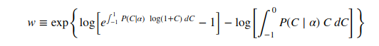
An equivalent integral version of @wigglemuse’s geometric Sharpe ratio:
w = \exp\left\{\log\left[ e^{\int_{-1}^{1}P(C\mid \alpha)\ \log(1+C)\ dC}-1 \right] - \log\left[\int_{-1}^{0} P(C\mid \alpha)\ C \ dC\right] \right\}
where I have used instead of the maximum drawdown, the expectation of the drawdown. You can use this if you think you understand the distribution, P, of correlations, C, as a function of the model/distribution parameters, alpha. For clarity here is an image of the equation.
1 Like
code didn’t really work out there
I thought we were supposed to be submitting code here. You think latex is too slow? I already submitted a request on support quite a while ago and there were several community members who voted it up. @slyfox even suggested an install.
Sure we should submit code, but as it is now latex is unreadable.
Related post / paper on left-tail persistence
@arbitrage There is a small mistake in the adj_sharpe function. The version of kurtosis used by default in scipy already has the 3 subtracted, so the formula you have is subtracting that 3 again and will give spurious results.
2 Likes
Thanks for these @arbitrage! You (or anyone) wouldn’t happen to have the python code for calculating feature exposure available? Both the way @bor1 described it (here) and max feature exposure that @richai talked about in today’s OHwA?
@player1 I’ve got something that might help, not sure if it’s exactly what they use on the Numerai tournament, but it’s helped me with the feature exposure evaluations. It does require the scipy.stats module.
from scipy import stats
import numpy as np

...

predictors = train.columns.values.tolist()
feature_pearson = []
feature_spearman = []
for i in range(len(predictors)):
	feature_pearson.append(stats.pearsonr(preds_valid, valid[predictors[i]])[0])
	feature_spearman.append(stats.spearmanr(preds_valid, valid[predictors[i]])[0])

print("*******")
print("Pearson:")
print("Feat. Max: \t", np.max(feature_pearson))
print("Feat. Exp: \t", np.std(feature_pearson))
print("Spearman:")
print("Feat. Max: \t", np.max(feature_spearman))
print("Feat. Exp: \t", np.std(feature_spearman))
So this is after you’ve got a list of your predictions that you can compare to the real target values in your validation set.
2 Likes
Brilliant, thank you! Here’s what I got with one of my models (IceShark).
*******
Pearson:
Feat. Max: 	 0.2025210097078443
Feat. Exp: 	 0.06394568577456082
Spearman:
Feat. Max: 	 0.19976677632974976
Feat. Exp: 	 0.0634932164568535
Max feature correlation of 0.2 seems quite high (too high), would you agree?
I’ve got very similar results for the maximum as that. I’ve not really concentrated on the max value. The mean was more important for me, but since @richai mentioned the max value yesterday I might start looking into it.
1 Like
It can be tough to get the max down to less than .15 or so, but as usual depends on what you are doing. To throw a wrinkle into it, a summary stat of feature exposure is useful but not necessarily accurate (AS “exposure”) because it just means your predictions are correlated to some feature over the time period you are measuring (or averaged over eras or whatever). But that does not necessarily mean you are over-relying on that feature (although it might and probably does actually). And if you look at the same stat for a different validation period, you might get a similar max but that doesn’t mean it is the same features that are reaching that max.
You are also trying to be correlated to the real targets after all, and if a feature happens to also be correlated to the targets during that period, then being correlated with such a feature is not a bad thing (for that period). In other words, if that feature stops being correlated to the targets, but your model goes happily along remaining correlated to the targets but not that feature, then that’s a good model and your correlation to that feature wasn’t a main causative factor. So if you really want to dive deep on feature exposure, you’d look at each feature in isolation and compare correlations between predictions and targets vs partial correlation between predictions and targets with the feature as control variable (effect removed in partial correlation) and then you’ll get a better idea what effect it is really having on your model. And you need to do that over different periods where that feature was both more and less correlated with the targets. Then you can see which features are relatively highly correlated with your predictions, and if it is the same features that remain so over time.
3 Likes
Feature exposure and max feature exposure (computed with pearson’s correlation coefficient on validation data) for example predictions: 0.0796 and 0.1013. Another data point from one of my models: (fe: 0.0582, max fe: 0.0793).
I got like 0.23 max FE for the example model using the above code. That’s with training on both Train and Val. Would Max FE go up by that much just by including Val in training? Or am I more likely doing it wrong?
The numbers I got for the example model were computed from the example_predictions.csv file that is a part of the weekly data download. Running the python example script also gives similar numbers (albeit slightly different, because of different random seeds) for me. I’d recommed trying to reproduce it without training on val.
I’ve attached a snipped version of the code that I use, abridged to reproduce my results for example predictions, below. Just run it in the directory with the unzipped contents of the weekly zip file and you’ll get the same results for example predictions as what I’d posted above.
import csv
import numpy as np
import pandas as pd

TOURNAMENT_NAME = "kazutsugi"
PREDICTION_NAME = f"prediction_{TOURNAMENT_NAME}"


def feature_exposure(df):
    df = df[df.data_type == 'validation']
    feature_columns = [x for x in df.columns if x.startswith('feature_')]
    pred = df[PREDICTION_NAME]
    correlations = []
    for col in feature_columns:
        correlations.append(np.corrcoef(pred, df[col])[0, 1])
    return np.std(correlations)


def max_feature_exposure(df):
    df = df[df.data_type == 'validation']
    feature_columns = [x for x in df.columns if x.startswith('feature_')]
    fe = {}
    for era in df.era.unique():
        era_df = df[df.era == era]
        pred = era_df[PREDICTION_NAME]
        correlations = []
        for col in feature_columns:
            correlations.append(np.corrcoef(pred, era_df[col])[0, 1])
        fe[era] = np.std(correlations)
    return max(fe.values())


def read_csv(file_path):
    with open(file_path, 'r') as f:
        column_names = next(csv.reader(f))

    dtypes = {x: np.float16 for x in column_names if
              x.startswith(('feature', 'target'))}
    df = pd.read_csv(file_path, dtype=dtypes, index_col=0)

    return df


if __name__ == '__main__':
    tournament_data = read_csv(
        "numerai_tournament_data.csv")
    example_predictions = read_csv(
        "example_predictions_target_kazutsugi.csv")
    merged = pd.merge(tournament_data, example_predictions,
                      left_index=True, right_index=True)
    fe = feature_exposure(merged)
    max_fe = max_feature_exposure(merged)
    print(f"Feature exposure: {fe:.4f} "
          f"Max feature exposure: {max_fe:.4f}")
PS: iPad + Blink + mosh + Wireguard VPN + wakeonlan = fun. 
3 Likes
Where does this magic number come from?
Is this the correlation from some basic estimator?
richard said that this number approximated their average trading costs
1 Like
I just realized that the max_feature_exposure implementation in my previous post is incorrect (it’s computing the max of each era’s feature correlation, instead of the max of each feature’s correlation with the predictions). Here’s the same code block with the correct implementation.
import csv
import numpy as np
import pandas as pd

TOURNAMENT_NAME = "kazutsugi"
PREDICTION_NAME = f"prediction_{TOURNAMENT_NAME}"


def feature_exposures(df):
    df = df[df.data_type == 'validation']
    feature_columns = [x for x in df.columns if x.startswith('feature_')]
    pred = df[PREDICTION_NAME]
    correlations = []
    for col in feature_columns:
        correlations.append(np.corrcoef(pred, df[col])[0, 1])
    return np.array(correlations)


def feature_exposure(df):
    return np.std(feature_exposures(df))


def max_feature_exposure(df):
    return np.max(feature_exposures(df))


def read_csv(file_path):
    with open(file_path, 'r') as f:
        column_names = next(csv.reader(f))

    dtypes = {x: np.float16 for x in column_names if
              x.startswith(('feature', 'target'))}
    df = pd.read_csv(file_path, dtype=dtypes, index_col=0)

    return df


if __name__ == '__main__':
    tournament_data = read_csv(
        "numerai_tournament_data.csv")
    example_predictions = read_csv(
        "example_predictions_target_kazutsugi.csv")
    merged = pd.merge(tournament_data, example_predictions,
                      left_index=True, right_index=True)
    fe = feature_exposure(merged)
    max_fe = max_feature_exposure(merged)
    print(f"Feature exposure: {fe:.4f} "
          f"Max feature exposure: {max_fe:.4f}")
Update 3rd September, 2020: The feature exposure metrics have changed slightly since I posted this. I’m leaving the code in this post intact, as I’d posted it earlier. Please refer to this post to find out more about the new feature exposure and max feature exposure metrics.
1 Like
I am new here and I am trying to understand the whole Numerai project yet, but for me it looks like a possible Risk Free interest rate. At least it makes sense to me. The idea would be to avoid considering profits that can be obtained without risk in the market. For instance, this helps to make your own sharpe ratios comparable over time when the risk free rate change.