MMC Calculation "Punishes" Originality During Meta-Model Burns

[master_key]

@sdmlm

All other things being equal, MMC should always increase with a decrease in corr to the meta model. E.g. two models, same exact corr on target, the model with a lower corr with the meta model should always have higher MMC. The current MMC formula does not satisfy this during negative meta model rounds as less corr with meta model decreases MMC.

So this is not really what we want. Take a case where the metamodel is in a burn period, scoring -0.05. Model A submits random noise, and scores -0.01. Model B submits a model that is strictly better than the metamodel, but very similar to the metamodel, scoring -0.04.

What you’re saying is we should reward this model A random noise because it looks unique and it did better than the metamodel. But it gave 100% unique information, and the result was negative. It should be punished. It made the metamodel strictly worse than it was before. Model B however made the metamodel strictly better, so it should be rewarded.

Looking only at correlation_score and correlation_w_metamodel can be very misleading in this way. The current MMC approach corrects this though, and only rewards for real added unique information.

The reason we see some models with low correlation get hurt worse in burn rounds is because they are actually not helpful signals in most cases

MMC is very difficult… you don’t play it just because you can submit a unique signal. Anyone can do that. You play it because you have something valuable that is currently either absent or underrepresented in the metamodel.

Still, your code example highlights a different part of MMC design. It seems like this is really a case of it being a 1-P model, and that information gets removed by neutralization, just as submitting the metamodel itself would. You could also form a similar example where you submit exactly a negative version of the metamodel, and boom you have something SUPER ORIGINAL (-1 corr with metamodel), and also scored +0.05 instead of -0.05! In your encoded example, that unique model was actually worse than simply submitting a negative metamodel in its entirety. But that’s not really original, it’s just market timing with a signal we already have. I can see some argument for rewarding that, but it’s not what we wanted to accomplish with MMC. Corr will already reward that timing ability proportionally to its value.

[sdmlm]

@master_key

What you’re saying is we should reward this model A random noise because it looks unique and it did better than the metamodel. But it gave 100% unique information, and the result was negative. It should be punished. It made the metamodel strictly worse than it was before. Model B however made the metamodel strictly better, so it should be rewarded.

I am a bit confused by this. How did model B make the metamodel strictly better? The current MMC formula doesn’t implement about how the metamodel is affected by the user’s predictions. Also, why are you saying model A is random noise? How would you know that? Based on this premise, then we should punish model A even when the meta model is positive, but then why even care about originality? Also, this is an extreme example/case, realistically most models are within 0.3 to 0.95 corr with the meta model, so they are def not random noise. Yet in negative meta model rounds, the more you go towards 0.3 corr with the meta model, the lower your MMC scores becomes.

[sdmlm]

@master_key

Looking only at correlation_score and correlation_w_metamodel can be very misleading in this way. The current MMC approach corrects this though, and only rewards for real added unique information.

This is also confusing. The current MMC does not say anything about how the meta model behaves in relation to a user’s model. It only cares about how a user’s model behaves in relation to the meta model (very different things). Again, when the meta model is negative, the more unique you are the lower your MMC score. It doesn’t have to be 0 or negative corr with the meta model.

[sdmlm]

@master_key

Still, your code example highlights a different part of MMC design. It seems like this is really a case of it being a 1-P model, and that information gets removed by neutralization, just as submitting the metamodel itself would. You could also form a similar example where you submit exactly a negative version of the metamodel, and boom you have something SUPER ORIGINAL (-1 corr with metamodel), and also scored +0.05 instead of -0.05! In your encoded example, that unique model was actually worse than simply submitting a negative metamodel in its entirety. But that’s not really original, it’s just market timing with a signal we already have. I can see some argument for rewarding that, but it’s not what we wanted to accomplish with MMC. Corr will already reward that timing ability proportionally to its value.

My code example was just to illustrate the MMC formula and it’s behavior under negative meta model rounds. There are plenty of real model examples (not 1-p etc) on this forum and the chat where simply having lower (not negative just a bit lower) corr with the meta model but higher corr on target leads to a lower MMC score during meta model negative rounds.

[lackofintelligence]

What you’re saying is we should reward this model A random noise because it looks unique and it did better than the metamodel. But it gave 100% unique information, and the result was negative. It should be punished. It made the metamodel strictly worse than it was before. Model B however made the metamodel strictly better, so it should be rewarded.

The only metric that you have for determining whether one model is strictly superior to another model is the correlation to the resolved scores. So if someone bets their bank on random noise, then it is because they believe that a strategy of random noise will be superior to any other strategy, especially in the context where we only report orderings and not magnitudes for our predictions, i.e., submitting random noise is the analogy of reducing the amplitude of predictions in the correlation to outcome context.

[master_key]

@sdmlm

Yet in negative meta model rounds, the more you go towards 0.3 corr with the meta model, the lower your MMC scores becomes.

This just isn’t necessarily true. For examples where you can find users who have lower corr_w_metamodel and lower MMC, you can also find users with lower corr_w_metamodel and higher MMC. It just depends on which way that independent vector faces with respect to the target.

If a model is very unique, but it’s still burning at the same time as the metamodel, why would we reward that model? A key point of MMC for us is finding signals which burn at different times. If your model is uncorrelated but burns at the same time as the metamodel, then it means that all of your uniqueness was for nothing . You just found a unique way to burn that no one else found. Not very helpful for us.

The problem with your analysis is you’re looking at the universe of users where
They are unique
AND there’s a burn period for the metamodel
AND the user still burned at the same time too.

The truth is that if you are unique, in general, you are more likely to be OK in a burn period. If you are burning at the same time while being unique, then it means you may have just managed to isolate a part of the metamodel responsible for the burning, and the rest of your signal didn’t save you.

Take this data for round 218 showing users who have roughly 30% corr with metamodel.

Then look at the data for round 218 showing users who have high corr with metamodel. Which group has better scores on average? Which group has higher MMC on average?

It should be clear that in this burn round, it was not necessarily better or worse to be unique. It only matters what type of uniqueness you have, whether it’s good uniqueness or bad uniqueness.

Being more unique definitely allows for higher magnitudes of MMC, in either direction. But your direction is still influenced by the quality of your signal with respect to the target.

[sdmlm]

@master_key

This just isn’t necessarily true. For examples where you can find users who have lower corr_w_metamodel and lower MMC, you can also find users with lower corr_w_metamodel and higher MMC. It just depends on which way that independent vector faces with respect to the target.

This is not the problem here. The problem is that, during meta model burns, 2 models with the same corr on target, one with lower corr_w_metamodel and one with higher corr_w_metamodel, the one with lower corr_w_metamodel will have lower MMC.

@master_key

If a model is very unique, but it’s still burning at the same time as the metamodel, why would we reward that model? A key point of MMC for us is finding signals which burn at different times. If your model is uncorrelated but burns at the same time as the metamodel, then it means that all of your uniqueness was for nothing . You just found a unique way to burn that no one else found. Not very helpful for us.

There are numerous examples of models with positive corr on target and negative MMC during negative meta model rounds.

@master_key

The problem with your analysis is you’re looking at the universe of users where
They are unique
AND there’s a burn period for the metamodel
AND the user still burned at the same time too.

Again the user doesn’t have to burn for this to happen and they also don’t have to be unique, the problem is that MMC is an increasing function of corr with the meta model during negative meta model rounds.

@master_key

The truth is that if you are unique, in general, you are more likely to be OK in a burn period. If you are burning at the same time while being unique, then it means you may have just managed to isolate a part of the metamodel responsible for the burning, and the rest of your signal didn’t save you.

Take this data for round 218 showing users who have roughly 30% corr with metamodel.

Then look at the data for round 218 showing users who have high corr with metamodel. Which group has better scores on average? Which group has higher MMC on average?

The data you posted actually proves my point.

As shown by previous forum posts and by @lackofintelligence mathematical note, MMC = CORR_user - CORR_WITH_METAMODEL * CORR_META_MODEL_ON_TARGET. Looking at this it is clear that MMC will increase with CORR_user , but decrease with CORR_WITH_METAMODEL .

From the data you posted for round 218:
user sunkay: -1% corr_target, 91% corr with meta model, 1.59% MMC
user souryuu: 0.25% corr_target, 31% corr with meta model, 1.33% MMC

As you can see, we gave user sunkay a larger MMC even though user souryuu has much better, positive corr on target.

Again, it is mathematically proven that MMC = CORR_user - CORR_WITH_METAMODEL * CORR_META_MODEL_ON_TARGET. Meaning that the users with low CORR_WITH_METAMODEL from your example data got MMC due to higher CORR_user, which offset the loss from CORR_WITH_METAMODEL * CORR_META_MODEL_ON_TARGET.

In any case, I think I’ve basically exhausted all possible arguments/examples I could give.

In the end it is what it is.

I really enjoy this tournament and have really tried my absolute best to improve it by trying my hardest to identify and explain this problem and ways to fix it.

If other users want to contribute to this please feel free, but I don’t think there’s anything else I could say on the matter.

[lackofintelligence]

For this data, what you should be looking at is the differences between MMC and CORR in relation to the correlation with the meta model. Let’s pick two points and compare. For purple who has the most unique model shown, the difference between MMC and CORR = 0.057 - 0.042 = 0.015. For the least unique model shown, rehoboam, the difference is -0.00555 - -0.02777 = 0.02222. So rehoboam is rewarded much more solely for being more like the meta model, which makes no sense as usual, especially since purple has a much better model in this round. All of this data seems to follow this trend except for a couple of outliers that suggest some other kind of oddities in this data.

[jackerparker]

There is almost no sense to compare correlation with the meta model between users. You can split your predictions into two parts - most confident and least confident, reverse the latter one and as the result - significant drop in correlation with meta model and almost the same correlation with real target. And the MMC right now exactly represents a “useful uniqueness” your model have.

Another example for the situation discussed in the beginning of this post: Users 1-5 have unique models with -0.01 Corr and 0 corr with MM. MM is based on these 5 predictions and results in -0.05 Corr.
User 6 has a model which is staked models from User 1-4 with -0.04 Corr and 80% corr with MM.
In the current MMC calculation system, Users 1-5 will get negative MMC values and User 6 will get high positive MMC. And all of that just sounds right.

[jackerparker]

There was feedback in the private messages which forced me to clarify my statements.

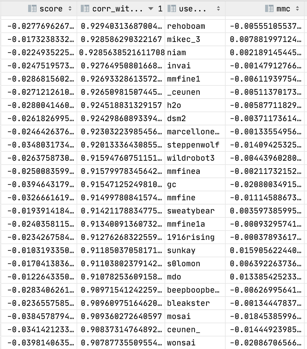
I believe that we cannot use any live data results as any justification of the theory discussed above. My point is that correlation with MetaModel is a completely wrong metric for model uniqueness. There are 4 example models in the attached code (based on the sdmlm’s code). First one is MM with -0.055 CORR performance . Second one is a true unique model with -0.036 CORR performance, 41% corr with MM, -0.066 MMC and -0.03 MMC-CORR value. The third one is a noisy “unique” model with -0.03 CORR performance, 43% corr with MM, -0.15 MMC and -0.12 MMC-CORR value. By the term noisy model I mean here that correlation was reduced mostly using part of predictions which does not correlate with target values. And the last, fourth model is highly correlated which is basically a noisy “unique” model with less artificial shuffles of predictions which does not correlate with target values. It has the same -0.03 CORR, 65% corr with MM, -0.075 MMC and -0.044 MMC-CORR value. So, truly unique model have the highest MMC and MMC-CORR metrics despite the worst raw CORR performance. Highest correlation model has better MMC and MMC-CORR metrics than noisy unique model. Both results provide me with the feeling that current MMC implementation is totally fine. And this “So rehoboam is rewarded much more solely for being more like the meta model, which makes no sense as usual, especially since purple has a much better model in this round. All of this data seems to follow this trend except for a couple of outliers that suggest some other kind of oddities in this data.” can be just explained by most of “unique” models in live data are fulfilled with a noise except “the couple of outliers” which are truly unique and useful models.

The only thing which makes me feel slightly less confident in my example is using 0.3 value in low_meta_corr_model array. So, any comments about that are appreciated.

Regards,
Mark

import numpy as np
import pandas
import scipy.stats

def spearmanr(target, pred):
    return np.corrcoef(
        target,
        pred.rank(pct=True, method="first")
    )[0, 1]

def neutralize_series(series, by, proportion=1.0):
   scores = series.values.reshape(-1, 1)
   exposures = by.values.reshape(-1, 1)

   # this line makes series neutral to a constant column so that it's centered and for sure gets corr 0 with exposures
   exposures = np.hstack(
       (exposures, np.array([np.mean(series)] * len(exposures)).reshape(-1, 1)))

   correction = proportion * (exposures.dot(
       np.linalg.lstsq(exposures, scores)[0]))
   corrected_scores = scores - correction
   neutralized = pandas.Series(corrected_scores.ravel(), index=series.index)
   return neutralized

def _normalize_unif(df):
    X = (df.rank(method="first") - 0.5) / len(df)
    return scipy.stats.uniform.ppf(X)

target = pandas.Series([0, 0, 0, 0,
          0.25, 0.25, 0.25, 0.25,
          0.5, 0.5, 0.5, 0.5,
          0.75, 0.75, 0.75, 0.75,
          1, 1, 1, 1])

meta_model = pandas.Series([1, 0, 0.25,
              1, 0.5, 0.75,
              0.5, 0.5, 1,
              0.75, 0.75, 0,
              0, 0.25, 0.25,
              1, 0, 0.25, 0.5, 0.75])
     
high_meta_corr_model = pandas.Series([1, 0, 0.25,
              1, 0.75, 0.5,
              0.5, 0.5, 0.75,
              0.75, 1, 0,
              0, 0.25, 0.25,
              0.75, 0.5, 1.0, 0.0, 0.25])

low_meta_corr_model = pandas.Series([0.3, 0.5, 0.75,
              1, 0.5, 0.75,
              0, 0, 1,
              0.75, 0.75, 0,
              0.25, 0.25, 0.5,
              1, 1, 0, 0.25, 0.25])

low_meta_corr_model_noise = pandas.Series([0.25, 0, 1,
              1, 0.75, 0.5,
              0.5, 0.5, 0.75,
              0.75, 1, 0,
              0, 0.25, 0.25,
              0.75, 0.5, 1.0, 0.0, 0.25])
   
# Meta model has raw corr with target of -5.5% (burning period)
meta_model_raw_perf = spearmanr(target, meta_model)
print(f"Meta_model performance: {meta_model_raw_perf}")

high_meta_corr_raw_perf = spearmanr(target, high_meta_corr_model)
high_meta_corr = spearmanr(meta_model, high_meta_corr_model)

print(f"High_meta_corr model cross-corr: {spearmanr(meta_model, high_meta_corr_model)}")
print(f"High_meta_corr model performance: {high_meta_corr_raw_perf}")


low_meta_corr_raw_perf = spearmanr(target, low_meta_corr_model)
low_meta_corr = spearmanr(meta_model, low_meta_corr_model)

print(f"Low_meta_corr model cross-corr: {spearmanr(meta_model, low_meta_corr_model)}")
print(f"Low_meta_corr model performance: {low_meta_corr_raw_perf}")


low_meta_corr_raw_perf_noise = spearmanr(target, low_meta_corr_model_noise)
low_meta_corr_noise = spearmanr(meta_model, low_meta_corr_model_noise)

print(f"Low_meta_corr_noise model cross-corr: {spearmanr(meta_model, low_meta_corr_model_noise)}")
print(f"Low_meta_corr_noise model performance: {low_meta_corr_raw_perf_noise}")


# MMC Computation
# All series are already uniform

# Neutralize (using forum post code for neutralization)
neutralized_high_corr = neutralize_series(high_meta_corr_model, meta_model, proportion=1.0)
neutralized_low_corr = neutralize_series(low_meta_corr_model, meta_model, proportion=1.0)
neutralized_low_corr_noise = neutralize_series(low_meta_corr_model_noise, meta_model, proportion=1.0)


# Compute MMC
mmc_high_corr = np.cov(target, 
                            neutralized_high_corr)[0,1]/(0.29**2)

mmc_low_corr = np.cov(target, 
                            neutralized_low_corr)[0,1]/(0.29**2)

mmc_low_corr_noise = np.cov(target, 
                            neutralized_low_corr_noise)[0,1]/(0.29**2)

print(f"MMC for non-original model: {mmc_high_corr}")
print(f"MMC for original model: {mmc_low_corr}")
print(f"MMC for original noise model: {mmc_low_corr_noise}")


print(f"MMC-CORR for non-original model: {mmc_high_corr-high_meta_corr_raw_perf}")
print(f"MMC-CORR for original model: {mmc_low_corr-low_meta_corr_raw_perf}")
print(f"MMC-CORR for original noise model: {mmc_low_corr_noise-low_meta_corr_raw_perf_noise}")

Meta_model performance: -0.05518254055364692
High_meta_corr model cross-corr: 0.6560590932489134
High_meta_corr model performance: -0.030656966974248294
Low_meta_corr model cross-corr: 0.4169347508497767
Low_meta_corr model performance: -0.03678836036909795
Low_meta_corr_noise model cross-corr: 0.4353289310343258
Low_meta_corr_noise model performance: -0.030656966974248308
MMC for non-original model: -0.07529413605357009
MMC for original model: -0.06688466111771676
MMC for original noise model: -0.15449965579823513
MMC-CORR for non-original model: -0.044637169079321797
MMC-CORR for original model: -0.030096300748618812
MMC-CORR for original noise model: -0.12384268882398683

[sdmlm]

@jackerparker you didn’t transform the predictions to standard uniform (my original example were at least discretely uniform). By making them standard uniform at the start of the code, you get vastly different results.
Basically just add this right after creating your predictions:

target = pandas.Series(_normalize_unif(target))
meta_model = pandas.Series(_normalize_unif(meta_model))
high_meta_corr_model = pandas.Series(_normalize_unif(high_meta_corr_model))
low_meta_corr_model = pandas.Series(_normalize_unif(low_meta_corr_model))
low_meta_corr_model_noise = pandas.Series(_normalize_unif(low_meta_corr_model_noise))

MMC-CORR for non-original model is the highest MMC-CORR…

import numpy as np
import pandas
import scipy.stats

def spearmanr(target, pred):
return np.corrcoef(
    target,
    pred.rank(pct=True, method="first")
)[0, 1]

def neutralize_series(series, by, proportion=1.0):
   scores = series.values.reshape(-1, 1)
   exposures = by.values.reshape(-1, 1)

   # this line makes series neutral to a constant column so that it's centered and for sure gets corr 0 with exposures
   exposures = np.hstack(
   (exposures, np.array([np.mean(series)] * len(exposures)).reshape(-1, 1)))

   correction = proportion * (exposures.dot(
   np.linalg.lstsq(exposures, scores)[0]))
   corrected_scores = scores - correction
   neutralized = pandas.Series(corrected_scores.ravel(), index=series.index)
   return neutralized

def _normalize_unif(df):
X = (df.rank(method="first") - 0.5) / len(df)
return scipy.stats.uniform.ppf(X)

target = pandas.Series([0, 0, 0, 0,
      0.25, 0.25, 0.25, 0.25,
      0.5, 0.5, 0.5, 0.5,
      0.75, 0.75, 0.75, 0.75,
      1, 1, 1, 1])

meta_model = pandas.Series([1, 0, 0.25,
          1, 0.5, 0.75,
          0.5, 0.5, 1,
          0.75, 0.75, 0,
          0, 0.25, 0.25,
          1, 0, 0.25, 0.5, 0.75])
 
high_meta_corr_model = pandas.Series([1, 0, 0.25,
          1, 0.75, 0.5,
          0.5, 0.5, 0.75,
          0.75, 1, 0,
          0, 0.25, 0.25,
          0.75, 0.5, 1.0, 0.0, 0.25])

low_meta_corr_model = pandas.Series([0.3, 0.5, 0.75,
          1, 0.5, 0.75,
          0, 0, 1,
          0.75, 0.75, 0,
          0.25, 0.25, 0.5,
          1, 1, 0, 0.25, 0.25])

low_meta_corr_model_noise = pandas.Series([0.25, 0, 1,
          1, 0.75, 0.5,
          0.5, 0.5, 0.75,
          0.75, 1, 0,
          0, 0.25, 0.25,
          0.75, 0.5, 1.0, 0.0, 0.25])


# Make uniform
target = pandas.Series(_normalize_unif(target))
meta_model = pandas.Series(_normalize_unif(meta_model))
high_meta_corr_model = pandas.Series(_normalize_unif(high_meta_corr_model))
low_meta_corr_model = pandas.Series(_normalize_unif(low_meta_corr_model))
low_meta_corr_model_noise = pandas.Series(_normalize_unif(low_meta_corr_model_noise))

   
# Meta model has raw corr with target of -1.5% (burning period)
meta_model_raw_perf = spearmanr(target, meta_model)
print(f"Meta_model performance: {meta_model_raw_perf}")

high_meta_corr_raw_perf = spearmanr(target, high_meta_corr_model)
high_meta_corr = spearmanr(meta_model, high_meta_corr_model)

print(f"High_meta_corr model cross-corr: {spearmanr(meta_model, high_meta_corr_model)}")
print(f"High_meta_corr model performance: {high_meta_corr_raw_perf}")


low_meta_corr_raw_perf = spearmanr(target, low_meta_corr_model)
low_meta_corr = spearmanr(meta_model, low_meta_corr_model)

print(f"Low_meta_corr model cross-corr: {spearmanr(meta_model, low_meta_corr_model)}")
print(f"Low_meta_corr model performance: {low_meta_corr_raw_perf}")


low_meta_corr_raw_perf_noise = spearmanr(target, low_meta_corr_model_noise)
low_meta_corr_noise = spearmanr(meta_model, low_meta_corr_model_noise)

print(f"Low_meta_corr_noise model cross-corr: {spearmanr(meta_model, low_meta_corr_model_noise)}")
print(f"Low_meta_corr_noise model performance: {low_meta_corr_raw_perf_noise}")


# MMC Computation
# All series are already uniform

# Neutralize (using forum post code for neutralization)
neutralized_high_corr = pandas.Series(neutralize_series(high_meta_corr_model, meta_model, proportion=1.0))
neutralized_low_corr = pandas.Series(neutralize_series(low_meta_corr_model, meta_model, proportion=1.0))
neutralized_low_corr_noise = pandas.Series(neutralize_series(low_meta_corr_model_noise, meta_model, proportion=1.0))


# Compute MMC
mmc_high_corr = np.cov(target, 
                        neutralized_high_corr)[0,1]/(0.29**2)

mmc_low_corr = np.cov(target, 
                        neutralized_low_corr)[0,1]/(0.29**2)

mmc_low_corr_noise = np.cov(target, 
                        neutralized_low_corr_noise)[0,1]/(0.29**2)

print(f"MMC for non-original model: {mmc_high_corr}")
print(f"MMC for original model: {mmc_low_corr}")
print(f"MMC for original noise model: {mmc_low_corr_noise}")


print(f"MMC-CORR for non-original model: {mmc_high_corr-high_meta_corr_raw_perf}")
print(f"MMC-CORR for original model: {mmc_low_corr-low_meta_corr_raw_perf}")
print(f"MMC-CORR for original noise model: {mmc_low_corr_noise-low_meta_corr_raw_perf_noise}")


Meta_model performance: -0.01503759398496236
High_meta_corr model cross-corr: 0.6796992481203005
High_meta_corr model performance: -0.04360902255639097
Low_meta_corr model cross-corr: 0.4195488721804511
Low_meta_corr model performance: -0.06766917293233085
Low_meta_corr_noise model cross-corr: 0.463157894736842
Low_meta_corr_noise model performance: -0.007518796992481184
MMC for non-original model: -0.034737792600909013
MMC for original model: -0.06384083997464719
MMC for original noise model: -0.0005764144386876333
MMC-CORR for non-original model: 0.008871229955481959
MMC-CORR for original model: 0.0038283329576836583
MMC-CORR for original noise model: 0.006942382553793551

[of_s]

Where, how and more importantly why was it simply assumed that a unique model is random noise?

[of_s]

Related new discussion on RC:

Numerai Community