Introduction
Following up on some exploratory work on simulating portfolios built from Numerai’s crypto meta model, I wanted to investigate a statistical risk factor model for the crypto market and apply the model to more realistic backtest of the TB100 portfolio. This is largely unexplored territory but there are several precedents coming from traditional portfolio theory applied to the equity market, from where I draw most of the tools here.
TB100 Portfolio
The “TB100” stands for “top and bottom 100”, which means to go long and short the top and bottom 100 assets each round, sorted by meta model score. Here is a portfolio simulation of this strategy. On each day we initiate equally weighted positions, long and short, which last for 20 days (the duration of our prediction targets).
Previously I had made a simplified version of the backtest for the TB10 simulation, where on each day we assume we earn the future 20 day log returns of each position. Keeping the position weights correct allows us to simulate this return stream which should be attainable in real life.
One thing to note is that we can only simulate tickers for which we have data (from Yahoo) and also we require to have the data for the 600 preceeding days of each trading date, in order to create our statistical risk model in the next section.
However this simulation falls short of clearly defining entry and exit prices, a portfolio cash account and positions, and the effect of overlapping 20 day trading periods. Because of this I put together a backtest which simulates trades and exact portfolios based on the close prices and meta model signal every day, in such a way that should replicate the idea from the simulation of log returns above. Here we plot the portfolio value, assuming the initial investment is 1.0.
Here we get about 9% return instead of the theoretical 14% above. But this is now realistic, where we can track individual transactions throughout the simulation.
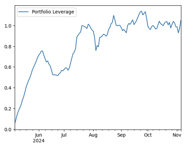
With this simulation we can also monitor things like cash account position and total portfolio leverage. We know from brief inspection that this portfolio makes most of the money short selling, and the crypto assets move a lot, so this greatly affects the leverage of the portfolio without and adjustments. The cash account stays at 1.0 for 20 days until our first round of trades expires, since each day we enter into equally weighted new positions, the new positions do not affect the cash account.
We also record the portfolio weights at each date and can then compute the churn of this portfolio over time.
The theoretical churn for this portfolio is 10% of net liquidity, since each day 5% new positions and 5% ending positions, since 1/20 (days) = 5%. Since we start with a portfolio value of 1$, the $ churn is also about 0.05 per day at the start.
Finally, if we have a risk model, we can compute portfolio exposures to market risk factors. This leads me to the next section.
Crypto Statistical Risk Model
The basic concept of an equity risk model is a linear factor model, that models cross-sectional market returns as a weighted linear combination of known factor returns. Visualize this with some pseudo code as follows.
return_asset_i = factor_0_beta_i * factor_return_0 + factor_1_beta_i * factor_return_1 + ... + noise
According to this model, on any date, we believe an asset’s return can be (to a certain extent) explained by the asset’s exposures (betas) multiplied by market factor returns. What the factors are is a big uncertain question. The idea of CAPM is that there is one general market factor, and all assets have exposure to this market factor, to some degree. The idea of the existence of the CAPM market factor is generally accepted mathematically and practically in the equity market.
However, common risk factor models tend to contain many more factors, leading some academics to describe the state of factor modeling in finance as a “factor zoo”. Traditional finance has approached this problem generally from two angles. The first is to assume we know some factor returns, and we fit a linear model by finding the betas to these known factor returns. This kind of modeling is driven by domain knowledge.
The an alternative technique is to assume that we don’t know what the factors are and we want to learn them from our data. This kind of factor model is usually called a statistical factor model, since it is created using statistical tools, namely PCA, or the singular value decomposition (SVD). I’ve always been intrigued by this second approach, thinking it must be informative and useful. This technique will decompose historical returns into principle components, where by the first component captures the largest portion of explained variance, and each successive component captures a diminishing portion. I decided to pursue this second approach in this article, to explore how to create and use a statistical factor model in the crypto market.
I consider this a work in progress and perhaps with more help from the community we can make this better.
The Process
The process is identical for each date throughout our simulation time span. Each time we must compile a set of usable historical return data. In my case I used the 20 day returns, and required 600 past days of return data. If we have N assets, this results in a (600 x N) matrix of asset returns. The SVD is then computed on this matrix, which results in the information we are looking for. Here we are most interested in factor returns and factor loadings (betas).
There are couple tricky parts here, in that the components of the SVD are unique up a sign. So as we shift our historical data set for every day that goes by, the (600 x N) matrix changes, because of changes of returns and also usable assets entering and exiting the universe. Every day the data is slightly different. I enforced that the direction of the first component always goes in a similar direction as the mean return of the market, since the first component is the largest market factor. We will see later it is very close to the mean return of the market. I also put in logic to keep the directions of the secondary factors (2nd component of higher) to be consistent.
Some Results
As we should expect, the first component of the SVD captures a factor that is almost identical to the mean return of the market, so we can think of this first risk factor as the “market return”, consistent with CAPM ideas, this statistical factor also shows that largest explained variance by far.
so for this date we can now rank the betas and we find that BTC does not have the largest beta, instead the largest beta is for a coin called SNS. We can confirm with some plots that indeed BTC differs from the market factor more than SNS.
With this technique we can also get the higher components of the SVD, and use them as risk factors too, in my test here, I used the first 3 components as risk factors. One thing to check is that the betas stay somewhat consistent over time, since the input data to the SVD changes as time goes by. Here we plot the beta rank of the first risk factor of BTC over time.
The beta ranges between the 25 and 27th percentile over the 5 months, this is pretty consistent. So now using this risk model we can compute portfolio exposures using asset and date - specific factor exposure to the top 3 factors, from our TB100 simulation above.
Risk Mitigation
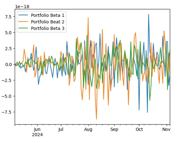
The last part of this article is to investigate mitigating portfolio risk by neutralizing our portfolio to these risk factors. What I tried here was to project the real-time portfolio onto the null space of the risk betas at each date, thus getting a portfolio not much different from our original, but now neutral to the risk factors. In theory this should smooth out our return stream. This is by way of making slight adjustment each day. This actually seems to work, slightly, resulting in a bit less than overall return than the original, but a higher Sharpe ratio, Here the non-annualized Sharpe is 0.1765, compared to 0.15 of the original. Here is the return stream and portfolio betas.
The slight increase to churn after this neutralization was minimal.
So there we have it, a market-neutral TB100 Crypto portfolio with statistical risk mitigation.
Code
Please find all code to replicate this simulation here.
Thoughts/Discussion
I meant this to be more of a starting point than an end in itself, so please let me know with any feedback. If you noticed I didn’t do any optimization here. I did try an idea to optimize the portfolio input vector at each date, instead of the naive equal weights, but then you still have the problem of exposures getting out-of-whack during the simulation period, and adjustment may still be required.
Also interested to see if any and point out some mistakes or bugs. I was maybe expecting the result of the risk neutralization to work better than it did.
With this framework, we can also apply other risk models just as long as we know how to compute the betas at each date, so this framework can be used to compare competing strategies and risk control ideas.


