In Signals, we have
- the ability to track targets on a per ticker basis through time
- new targets updated every week for recently resolved eras
This allows us to use time series methods that aren’t possible in the Classic Tournament. In fact, this means we can even predict future targets and participate in Signals without having to use any external data at all–using only a ticker’s previous targets. To be sure, we shouldn’t expect to get great scores, but it’s a fun exercise and what we learn can likely be applied to modeling paired with other external data. Since targets are bucketed measures of transformed returns, you can also think of this as a type of momentum or reversal prediction model.
Targets exploration
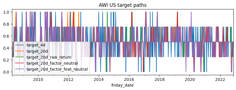
First, let’s pick a random ticker and plot its targets over time. As we know, targets only take on 5 possible values: [0, 0.25, 0.5, 0.75, 1], so the plot doesn’t seem to contain all that much information:
But if we take a rolling mean, we can start to see some patterns and trends potentially emerge. Indeed, maybe we see how this can be treated as a pure time series problem:

Let’s look at some autocorrelation plots to see if there are any overall relationships in the time series data. Autocorrelation plots are important in time series analysis because they show the relationship between a variable and itself at different time intervals. This can help identify patterns and trends in the data that can be used for forecasting. For example, if a time series has a strong positive autocorrelation at a lag of 2, it indicates that the current value is likely to be similar to the value 2 time periods ago. This information can be used to build better predictive models.
Since we have 10s of thousands of tickers in the dataset, we have to compute each ticker’s autocorrelation separately. Then, we can plot the distributions of those autocorrelations for each lag:

In our case it’s no surprise that we have significant autocorrelation up until lag_4. That’s because each era starts weekly, but has a duration of one month. For the same reason that we need to make sure our train/test set splits have at least a four week gap in Classic, we need to make sure that we’re using fully resolved targets as data for this exercise.
There may also be a hint of negative autocorrelation at lag_5 so this might suggest the targets start to trend in the opposite direction (reversal or mean reversion) after a month.
Now that we have some sense of what the targets look like, we can try some forecasting methods, starting simple and getting progressively more fancy.
Baseline lag prediction
For the most naive possible baseline, our predictions will be a ticker’s target as of 5 lags ago (this is also the most recent available target in the weekly validation data updated by Numerai at round open). But, since the autocorrelation plot suggests there may be negative autocorrelation at lag_5, we’re going to flip the sign so that our predictions are: \hat{Y_t} = 1 - Y_{t-5}
To visualize and try to gain an intuition of what’s going on, this chart shows a random ticker’s rolling target over time, it’s lagged target (as of 5 eras ago), and the inverse of that lag, which we’ll use as our predictions. For visualization purposes, this is the rolling mean of this ticker’s targets, but our actual values for all modeling are the discrete target values for that era.

Now that we have baseline predictions, let’s see if this can actually translate into any scoring. Nothing particularly great, but also looks like we may be on to something–it’s certainly not random:

Averaged lag predictions (rolling mean)
Instead of just taking lag_5, maybe we can do slightly better if we average the lag_5, lag_6, and lag_7? Like the simple baseline, we’ll also take the 1-p version assuming a reversal strategy.
\hat{Y_t} = 1 - \frac{(y_{t-5} + y_{t-6} + y_{t-7})}{3}
Simple univariate linear model (autoregression)
Now let’s add some modeling in with a simple linear regression. This is sort of a pseudo time-series model because 1) we have not verified many assumptions needed for proper timer series models and/or 2) we’re not taking the order of the lags into account. Instead, we’re using the time series lags to create cross-sectional features. We’ll use the lags and build a very simple linear regression to predict the current time step. Specifically:
\hat{Y_t} = \beta_1Y_{t-5} + \beta_2Y_{t-6} +...+\beta_{16}Y_{t-20}
Ideally, if the assumption we’ve been operating under–that lag_5 should have a negative reversal–is true, we would hope that the linear model learns a negative coefficient for \beta_1. As it turn out, we do:

Traditional time-series models
At this point you can and probably should use more traditional time series models. The linear model above is a butchered version of VAR and ARMA models, but I skipped them for now because I’d have to use statsmodels or R. These models also tend to require data transformations due to additional assumptions about the nature of your time series. Mostly, I just don’t like them.
Multivariate non-linear model (xgboost)
Now that we have 4 new targets in Signals, lets add those lags into the equation as if they were just more features. So instead of just using the lagged target_20d, we can also use the lagged target_20d_raw_returns, target_20d_factor_feat_neutral, and target_20d_factor_neutral
Features: lag_features = ['target_20d_lag5', 'target_20d_factor_neutral_lag5', 'target_20d_factor_feat_neutral_lag5', 'target_20d_raw_return_lag5', ... , 'target_20d_lag15', 'target_20d_factor_neutral_lag15', 'target_20d_factor_feat_neutral_lag15', 'target_20d_raw_return_lag15',
Target: target_20d
Then, we’ll simply train an xgboost regressor as if it were a cross-sectional problem:
model = XGBRegressor()
model.fit(train_df[lag_features], train_df["target_20d"])
LSTM
With the LSTM (RNN), we’re getting into some more heavy duty time series modeling. What’s nice about the LSTM model is that it takes the order/sequence of lags into account, where the model knows which lag follows which lag and, since it’s a neural net, in its latent space it’s computing more features about how the lags interact with one another. Moreover, we can relax a lot of assumptions needed in more classical time series modeling.
In this case, we’ll use 15 lags of all the targets to predict target_20d. With a “many to one” RNN modeling approach, our LSTM network looks a bit like this, where Y_t is target_20d and X_i, X_j, etc. are other targets (used as more features like in the xgboost example above) like target_factor_feat_neutral and target_raw_returns:

Evaluation
Now that we have 5-6 good prediction frameworks, ranging in increasing orders of complexity, let’s submit our predictions to Numerai and pull the diagnostics back so we can look at our fully neutralized correlation scores against the target we were trying to optimize: target_20d:


As it turns out, although it rarely does, as we keep getting fancier, our scores keep getting better!
A note on neutralization
This exercise has also been helpful in seeing the effects of Numerai’s scoring process. When we submit our Signals predictions, we are neutralized to a set of blackbox features before our final correlation scores are computed. In many cases using external data as features, I have seen this neutralization process improving correlation scores from local scoring to diagnostic (Numerai) scoring. In this case, neutralization has a large negative impact on correlation scores. This makes some sense since we are only using targets provided by Numerai, which are ostensibly constructed by the very features we are then being neutralized against. My intuition is that this method of time series modeling using only the Numerai provided targets is 1) as close as possible to also using Numerai’s internal features and 2) also would be heavily exposed to a momentum/reversal factor that we are likely already being neutralized against.
Here is an example with an LSTM model that gets a .0159 local correlation score (pre-neutralization) which then gets a .0102 diagnostics correlation score (post-neutralization). We add random predictions as a baseline measure:


Conclusion
We’ve been able to (seemingly) build semi-performant models for Signals without using any data at all! Starting with a simple baseline prediction of using the inverse of a ticker’s most recently resolved target and moving all the way to a recurrent neural net using multiple targets, it seems as though it’s entirely possible to participate in Signals using just the targets alone. While these models may not be able to achieve high scores on their own, they may be able to provide valuable insights when used in conjunction with external data. Overall, this exercise highlights the potential for using time series methods in Signals and the benefits of the new targets available in this tournament.